Linear Regression

1. Model Representation / Hypothesis function

The purpose of the model $h_{θ}$ is to predict output values $h_{θ} (x)$ from unseen input values $x$ (the features), using knowledge $θ$ extracted from a set of data for which the output values $y$ are already known.

Univariate Linear Regression model

The hypothesis function $h_{θ}$ of a Univariate Linear Regression is trying to map a single input value (the $x$ 's) to a single quantitative output value ( the $y$ 's or $h_{θ} (x)$ ) and it has the following format:

h_{θ} (x) = θ_{0} + θ_{1} x + ε

ε represents the errors made by the model – it accounts for the fact that the model won't perfectly retrieve the original $y$ values : $h_{θ} (x_{i}) \approx y_{i}$

The vector of errors ε has a normal distribution with a mean equal to 0 and an unknown variance (or covariance in a multivariate model).

Multivariate Linear regression model

The hypothesis function $h_{θ}$ of a Multivariate Linear Regression is trying to map multiple input values (the $x$ 's) to a single quantitative output value (the $y$ 's or $h_{θ} (x)$ ) and it has the following format:

h_{θ} (x) = θ_{0} + θ_{1} x_{1} + . . . + θ_{n} x_{n} + ε

$\begin{aligned} with n & = the number of features \\ x_{0} & = 1 (removed for convenience of notation) \\ ε & = the error made by the model \end{aligned}$

Using the matrix multiplication representation, this multi-variable hypothesis function can be concisely represented as:

h_{θ} (x) = [\begin{matrix} θ_{0} θ_{1} . . . θ_{n} \end{matrix}] [\begin{matrix} x_{0} \\ x_{1} \\ ⋮ \\ x_{n} \end{matrix}] + ε = θ^{T} X + ε

Optimizing the parameters

In order to build a model $h_{θ}$ one must find the $θ$ parameters. And this is done using a Cost function along with an Optimization method

2. Cost function

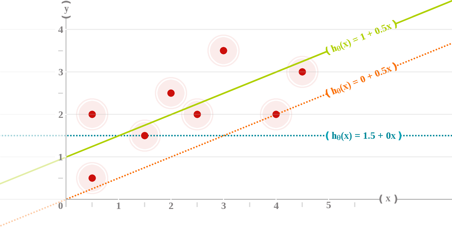
A cost function (or objective function) is a mathematical criterion used to measure how well the hypothesis function performed to map training examples to correct outputs.

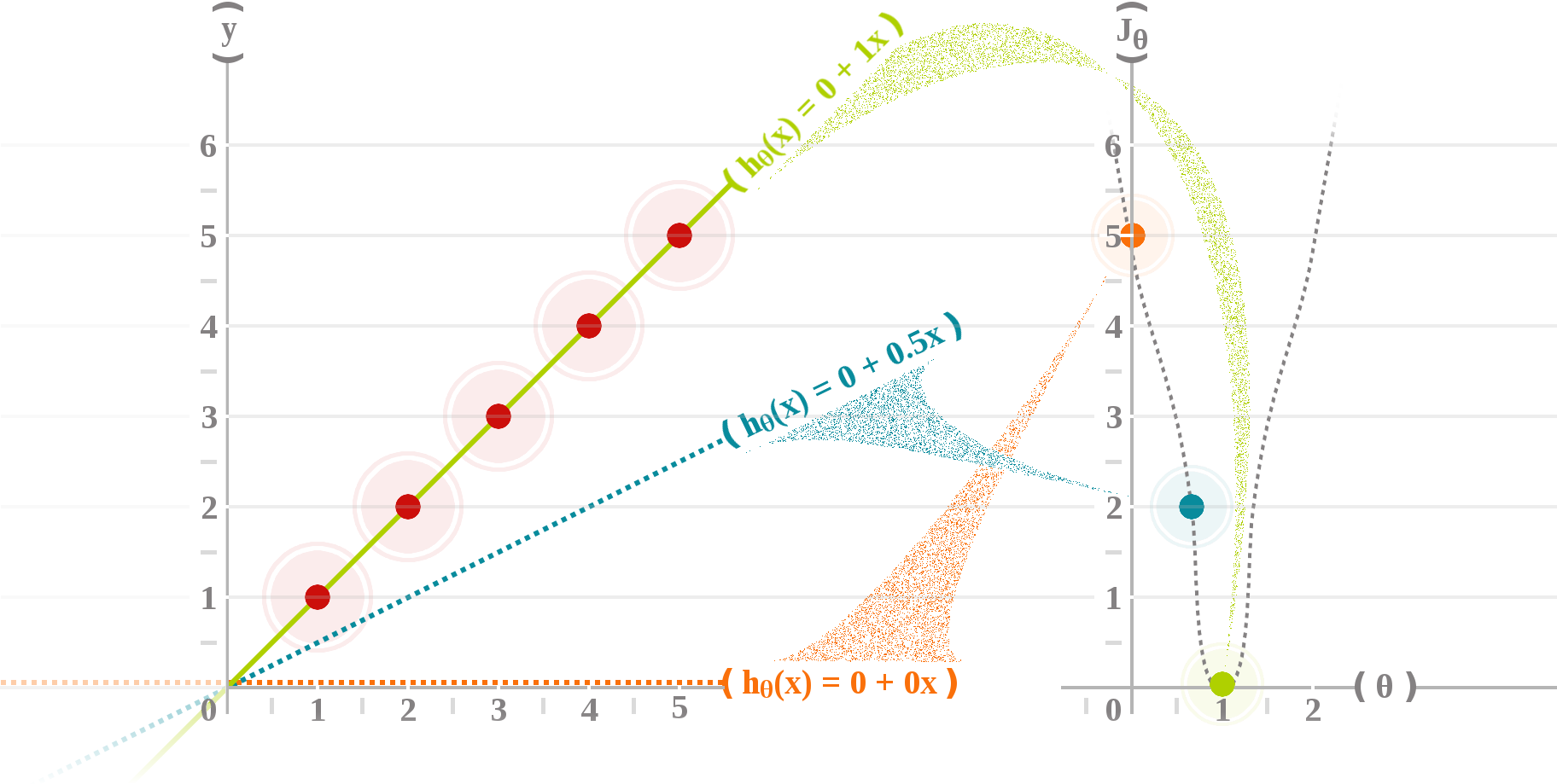
In the best case, the line passes through all the points of the dataset and the cost $J (θ) = 0$ (measured on the CROSS VALIDATION SET while selecting the model, then on TEST SET for final verification).

Cost functions for logistic regression problems includes :

Mean Error (ME),
Mean Squared Error (MSE),
Mean Absolute Error (MAE),
Root Mean Squared Error (RMSE),
Root Mean Squared Logarithmic Error (RMSLE),
etc.

In practice, the most common cost functions are the Mean Squared Error (MSE) in production (e.g. OLS or Gradient Descent) and the Root Mean Squared Error (RMSE) in analysis. Both lead to the same result, but MSE has one less step, so it's slightly faster, and RMSE has the advantage of having the same unit as the values plotted on the vertical axis and is easier to interpret.

The maximum likelihood estimation is another kind of objective function that is often used in practice. But when such an objective function is used, the goal is to maximize it rather than minimize it.

3. Optimization methods

To build the model $h_{θ}$ and use it to predict output values $h_{θ} (x)$ from unseen input values $x$ , one must find the $θ$ parameters.

This process of finding the values for which the error $ε$ made by the model gives a minimum value is called optimization.

And when it comes to solving such problems there exists both analytical and numerical approaches.

The analytical approach

An analytical solution involves framing the problem in a well-understood form and calculating the exact solution without using an iterative method.

In the case of a linear regression the method that is usually used is the Ordinary Least Squares (OLS) which will compute the $θ$ parameters with simple formulas, but it might be very slow with large datasets.

The numerical approach

A numerical solution means making guesses at the solution and testing whether the problem is solved well enough to stop iterating.

In the case of a linear regression the method that is usually used is the Gradient Descent which will iterate over the $θ$ parameters until it finds the lowest value $ε$ for the error made by the model.

This technique is a little excessive for univariate regression (as OLS is simpler), but its definitely useful for multivariate regression.

Advanced Optimization

There exists several algorithms to optimize the $θ$ parameters that are more sophisticated than using Gradient Descent.

Here is a short list of the most often used optimization algorithms:

Conjugate Gradient
BFGS (Broyden–Fletcher–Goldfarb–Shanno)
L-BFGS (Limited-memory BFGS)

These optimization algorithms are usually faster, and they remove the hassle to manually pick $α$ . But in return, they are more complex to implement and it is usually highly recommended to use pre-written functions available in most machine learning libraries.

OLS (Normal Equation) vs Gradient Descent

OLS (Normal Equation)	Gradient Descent
No need to choose $α$	Need to choose $α$
No need to iterate	Needs many iterations
Find exact solution (most of the time...)	Makes guesses
No need to feature scaling	Feature scaling should be used
Slow if $n$ is larger than 10000	Works well when $n$ is large
$O (m n^{2}) + O (n^{3}) \approx O (n^{3})$	$O (k n^{2}) + O (m n^{2}) \approx O (n^{2})$ (for vectorized version) $O (n m k)$ (for non-vectorized version)

$\begin{aligned} with n = & the number of features \\ m = & the number of samples \\ k = & the number of iterations / steps of the gradient descent \end{aligned}$