Gradient Descent
The gradient descent is an iterative method used to automatically guess the optimal θ parameters of
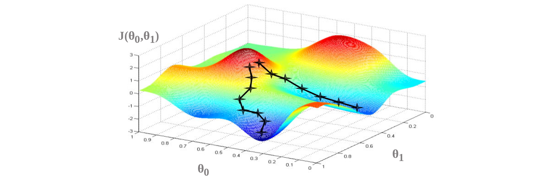
The idea is to take repeated steps in the opposite direction (when we try to minimize) of the approximate gradient of the function at the current point (because this is the direction of steepest descent), until it doesn't change anymore.
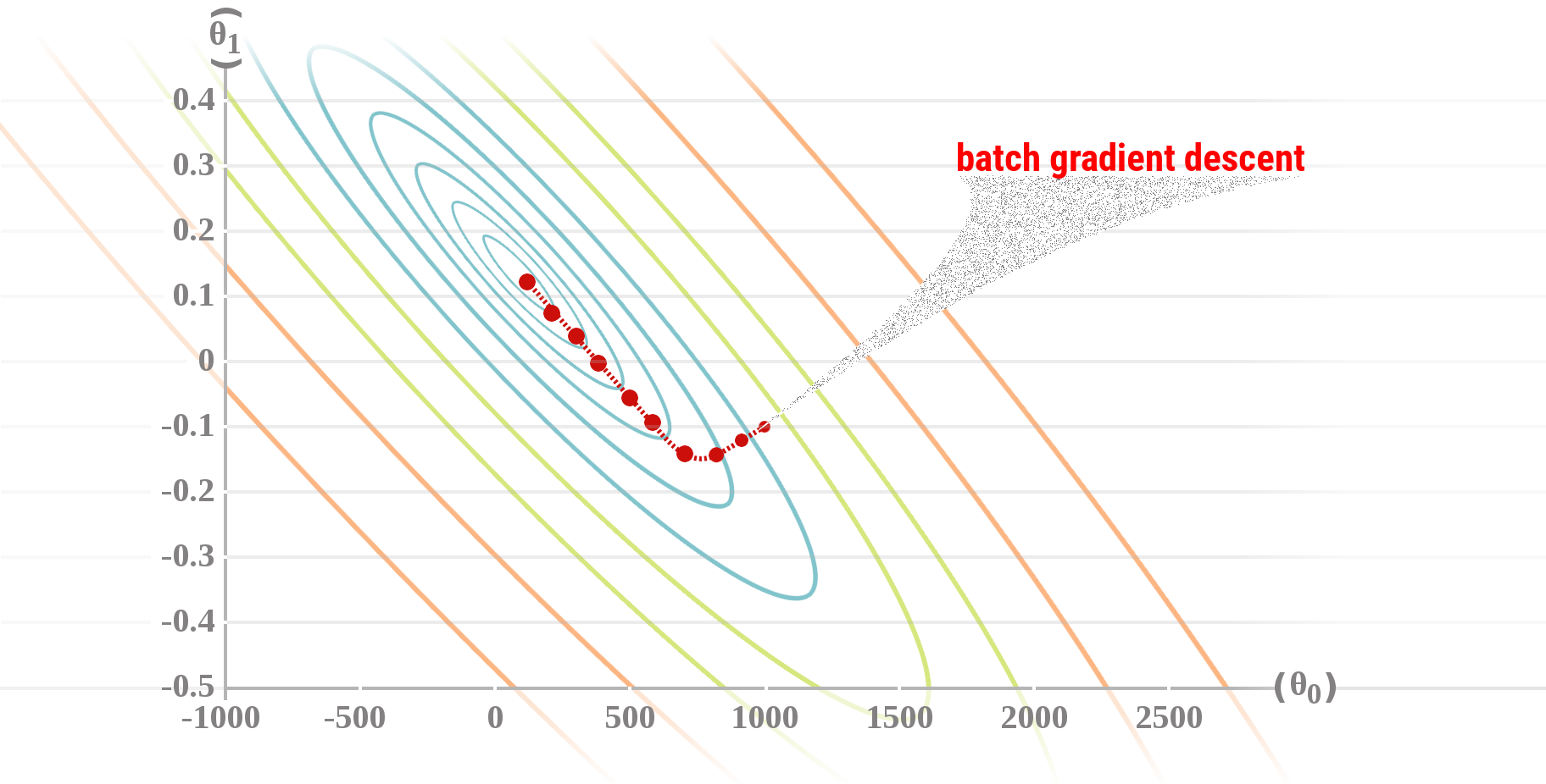
However, the gradient descent doesn't guarantee to find the global optima (the best parameters), and it can end-up in a local optima or another one depending on the starting point.
⚠️ It is recommended to use feature normalization to speed up the descent.
Four steps gradient descent example
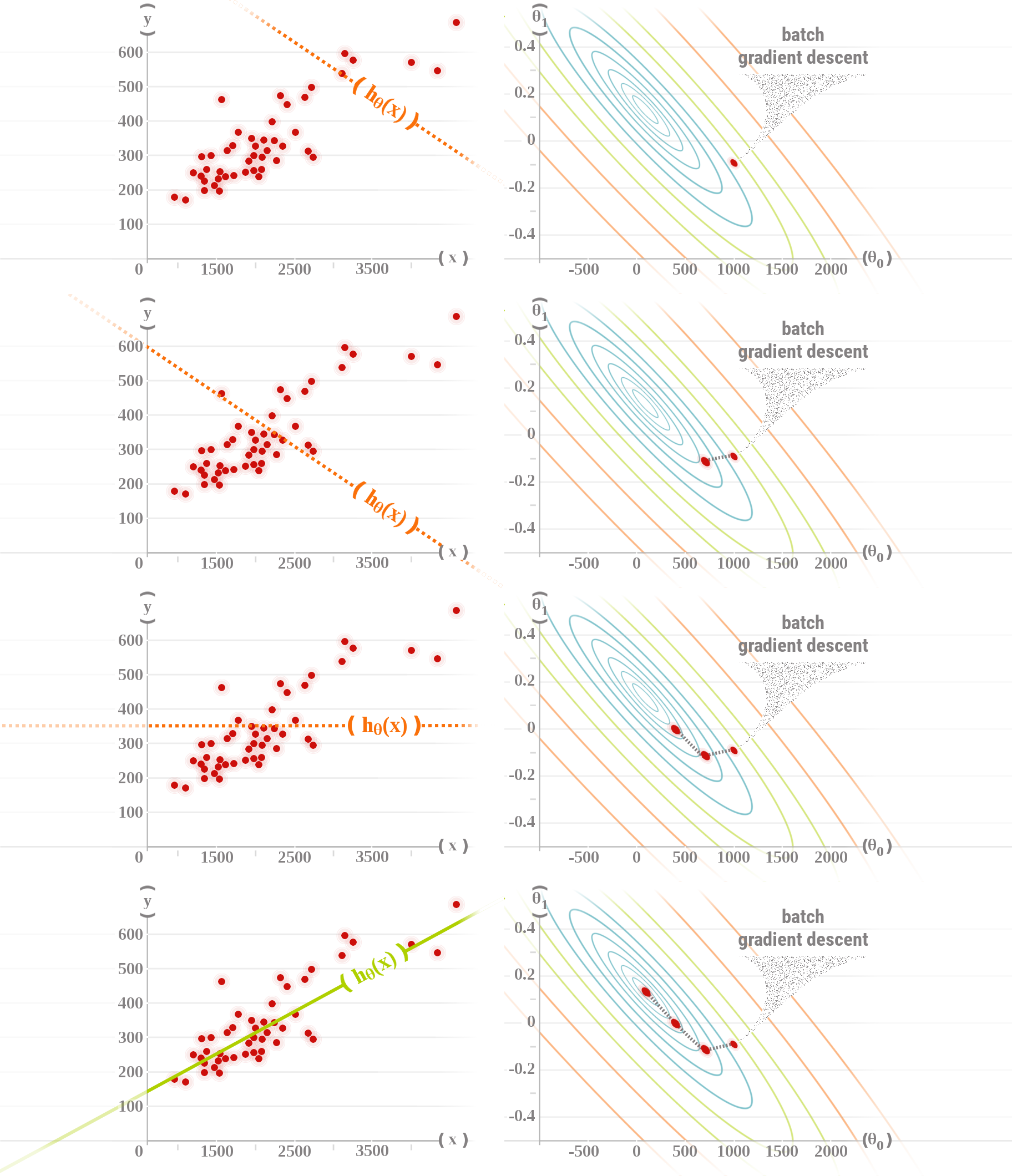
General Batch Gradient Descent algorithm
Normally, the derivative of the Mean Squared Error (MSE) cost function is as follows:
But if the cost function expression is already divided by 2 (see Mean Squared Error (MSE)), there is no need to do it again, and the formula becomes:
Batch Gradient Descent for univariate linear regression
Batch Gradient Descent for multivariate linear regression
Vectorized Batch Gradient Descent
The “default” gradient descent algorithm is the batch gradient descent algorithm which uses all the TRAINING EXAMPLES training examples available.
⚠️ TODO : Add other types of gradient descents HERE.
Debugging Gradient Descent
The simplest way to debug a gradient descent is to make a plot with the number of iterations and the Cost function
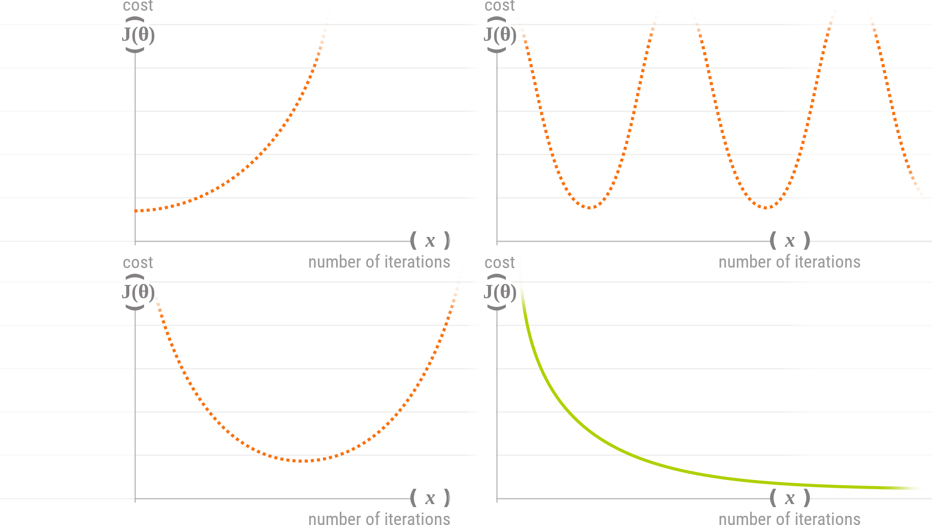
The learning rate
- If the learning rate
is too large, (like the ...orange... lines above) the gradient descent will have difficulties converging. - If the learning rate
is too low, the gradient descent will eventually converge, but it will take time... - If the learning rate
is just right, the gradient descent will be in its best configuration to quickly converge.
So, one good way to choose
is to start with a small value and to progressively increase it by almost 3 (… 0.001, 0.003, 0.01, 0.03, 0.1, 0.3, 1 …) as long as do not increase.